The goal of this project is to derive actionable insights to convert casual riders of the fictional Cyclistic Bike-Share company into annual members and provide other recommendations for the improvements of current business models. While considering the business inquiries and characteristics of data, I used R to clean and prepare the database and specially used the functions ggplot for some basic analysis. Then, I move the database to Tableau for visualisation.

Background
A successful bike-share programme operated by Cyclistic was introduced in 2016 with a fleet of 5,824 bicycles that are tracked and secured into a system of 692 stations throughout Chicago. The bikes may at any time be released from one station and brought back to any other station in the network. Members are those who have an annual membership, whilst casual users are those who just utilise single rides or full-day passes. The marketing director wants to increase the number of annual subscriptions because they are more profitable than day or single-ride passes.
The marketing team will create a new marketing plan to turn occasional riders into yearly subscribers. My primary responsibility on the team as a junior data analyst is to deliver engaging data insights and expert data visualisations. The key data analysis steps are as followed: Ask, Prepare Process, Analyze, Share, Act (In the future).
Ask
How do annual members and casual riders use Cyclistic bikes differently?
Why would casual riders buy Cyclistic annual memberships?
How can Cyclistic use digital media to influence casual riders to become members?
Prepare
The dataset was acquired from https://divvy-tripdata.s3.amazonaws.com/index.html. Motivate International Inc made the data available under this [license] (https://ride.divvybikes.com/data-license-agreement). For this project, I downloaded data for twelve months (August 2021 to August 2022) in CSV (comma-separated values) format, and each file contains 13 columns. The dataset passes the ROCCC Analysis, it is reliable (not biased), Original (locate the original public data), Comprehensive (key information is included), Current (monthly updated) and Cited.
Installing and loading necessary packages, and setting File Directory
library(ggplot2)
library(dplyr)
library(tidyverse)
setwd("C:\\Users\\desktop\\GOOGLE COURSE 8 DATABASE\\12 months of cyclistic trip data")
Import data and merge data into a data frame
Aug21 <- read.csv("202108-divvy-tripdata.csv")
# do the same for other 11 files
tripdata<- rbind(Aug21,Sep21,Oct21,Nov21,Dec21,Jan22,Feb22,Mar22,Apr22,May22,Jun22,Jul22,Aug22)
Process
Before cleaning the data, review the data frame generally.
# General review
tripdata
# see the column names of data
colnames(tripdata)
# no. of rows
nrow(tripdata)
# total NA values
sum(is.na(tripdata))
# See list of columns and data type
str(tripdata)
# Statistical summary of data
summary(tripdata)
 </p> Do some cleaning and processing for the data
# Remove NA value
tripdata<- na.omit(tripdata)

# check duplicate ride id
sum(duplicated(clean_data$ride_id))

# check the consistentcy of data formats
start<-as.POSIXlt(tripdata$started_at, tz = "","%m/%d/%Y %H:%M")
start<- data.frame(start)
start<- (start[1:nrow(na.omit(start)),])
start<- data.frame(start)
start1<-as.POSIXlt(tripdata$started_at, tz = "","%Y-%m-%d %H:%M")
start1<- data.frame(start1)
start1<- (start1[(nrow(start)+1):nrow(start1),])
start1<-data.frame(start1)
names(start)<- "start"
names(start1)<- "start"
start_time<- (rbind(start,start1))
tripdata$started_at <- NULL
tripdata['started_at']<- start_time
# the same for the column ended_at

# Adding a column for Ride length
ride_length<-difftime(end_time[,],start_time[,],unit="mins")
ride_length<-data.frame(ride_length)
tripdata<- cbind(tripdata,ride_length)
# check the uncommon ride length
clean_data <- tripdata%>% filter(ride_length>0)

# Adding columns for the day of the week
Tripdate<-as.Date(clean_data$started_at)
clean_data<-cbind(clean_data,Tripdate)
# In some cases, the language setting must be changed to ensure the function operation
Sys.setlocale("LC_TIME", "English")
weekday<-weekdays(clean_data$Tripdate)
weekday<-data.frame(weekday)
clean_data<-cbind(clean_data,weekday)

# view the data frame, and write file to path
view(clean_data)
write.csv(clean_data,"clean_data.csv", row.names = FALSE)

Analyze
In this step, the organized and formatted data is used for calculations and further aggregated, and a variety of charts and tables are generated to identify trends and relationships. Calculation
# calculate the average ride length, and the extreme value of duration in days
cat('average ride length: ', mean(clean_data$ride_length), "mins")
cat('maximum rides duration: ', round(max(clean_data$ride_length)/60/24), "days")
# average ride length: 17.89555 mins
# maximum rides duration: 29 days
# count the total number of membership and causual users,and show the ratio
clean_data%>% group_by(member_casual)%>% summarise(n=n())%>% mutate(percent = n*100/sum(n))
# count the total number of bike types,and show the ratio
clean_data%>% group_by(rideable_type) %>% summarise(n=n())%>% mutate(percent = n*100/sum(n))
# Useage in different weekdays
clean_data$weekday<- factor(clean_data$weekday)
weekday_table<- clean_data%>% group_by(weekday)%>% summarise(n=n())%>% mutate(percent = n*100/sum(n))


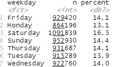
Aggregated
# The average ride length filter by member or casual
bar<-clean_data%>% group_by(member_casual)%>% summarise(avg_ride_length=mean(ride_length))
# The three different bike types filter by member of casual
rideable_type<-clean_data%>% group_by(rideable_type,member_casual) %>% summarise(n=n())%>% mutate(percent = n*100/sum(n))
# Users preference on differnt types of bike
member_type<-clean_data%>% group_by(member_casual,rideable_type) %>% summarise(n=n())%>%mutate(percent = n*100/sum(n))


Data display in general visual properties
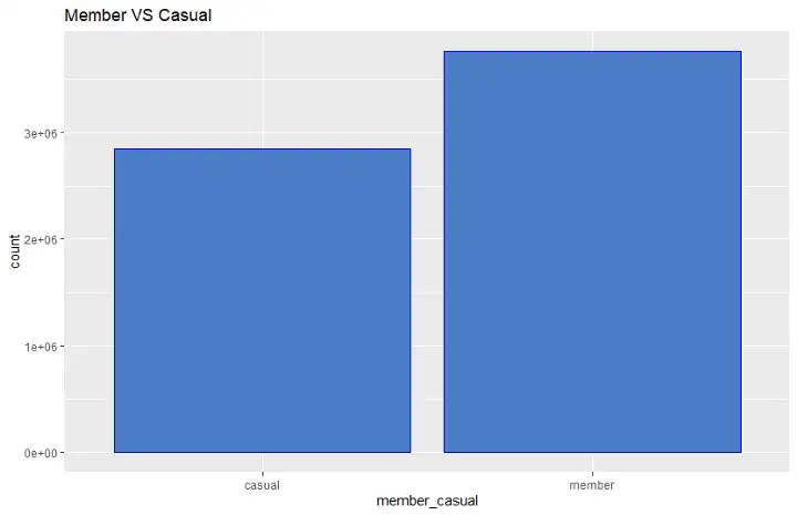
# Number difference in member or casual users
ggplot(data = clean_data,mapping= aes(x= member_casual)) +geom_bar() + labs(title="Member VS Casual")
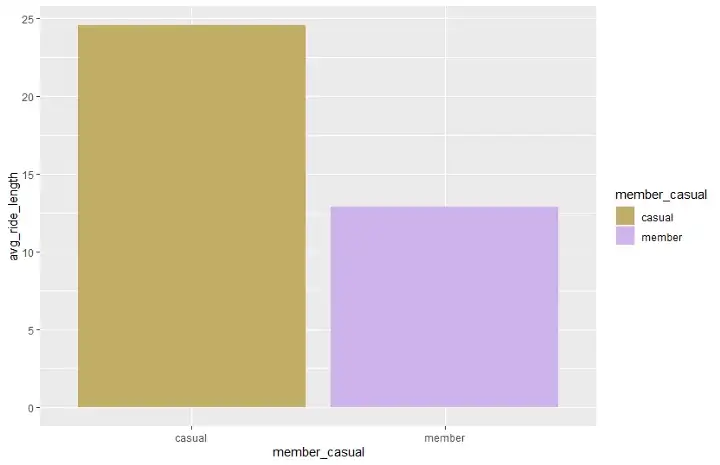
#the difference in ride length
ggplot(bar, aes(x = member_casual, y = avg_ride_length, fill =member_casual))+geom_col()+ scale_fill_manual(values = c("#c2ad64", "#cdb2ec"))
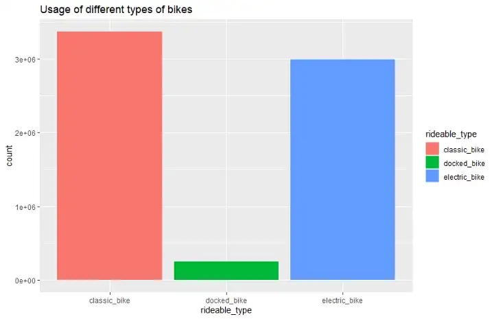
# Usage of different types of bikes
ggplot(data = clean_data,mapping= aes(x= rideable_type,fill=rideable_type)) +geom_bar() + labs(title="Usage of different types of bikes")
# Filter the usage by member or casual users
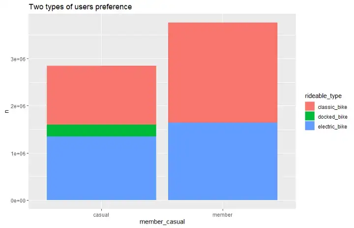
ggplot(data = as.data.frame(member_type),mapping= aes(x= member_casual, y=n, fill =rideable_type)) +geom_bar(stat = 'identity') + labs(title="Two types of users preference")
# Usage in different weekday
ggplot(data = clean_data,mapping= aes(x= weekday)) +geom_bar() + labs(title="Usage in different weekday")
# Bike usage pattern of casual users
casual_users<-clean_data%>% filter(member_casual == 'casual')%>%group_by(weekday,rideable_type)%>% summarise(n=n())%>% mutate(percent = n*100/sum(n))
ggplot(data= casual_users, mapping= aes(x= weekday, y=n, fill =rideable_type)) + geom_bar(stat = 'identity')+scale_fill_manual(values = c("#A8E6CE", "#DCEDC2","#FFD3B5"))
# Repeat the function for members to get bike usage pattern of members
# General filter by members and casual users
ggplot(data = clean_data,mapping= aes(x= weekday, fill = member_casual)) +geom_bar() +facet_wrap(~member_casual)+theme(axis.text.x = element_text(angle = 60, hjust =1))+scale_fill_manual(values = c("#A8E6CE", "#DCEDC2"))
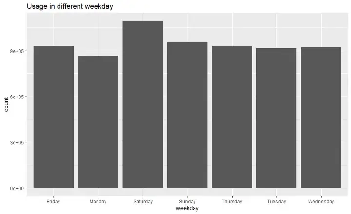


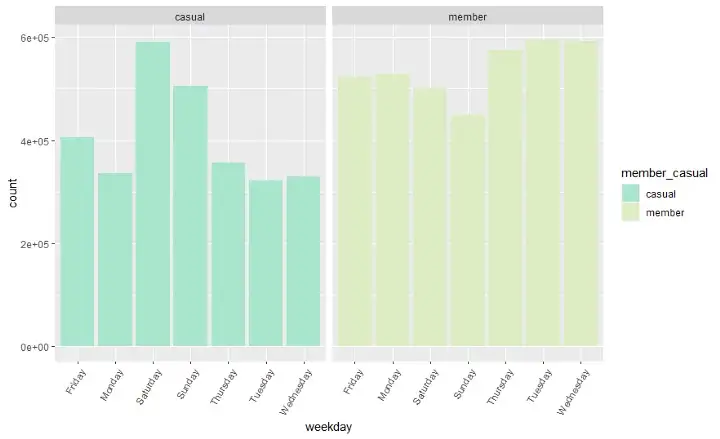
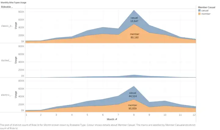
The main user type is still member, but casual users generally ride for longer distances. Classic Bike is preferred to Electric Bike, and the docked bike is seldom be used. Members prefer classic bike and never use docked bike, and casual users do not show an obvious preference between the two main ride types. Member’s usage is particularly lower on weekdays compared with other days. The customer group of members are more likely to be commuters. Casual user usage, in contrast, is much higher during the weekend.
Further data processing will be conducted in Tableau, Click here to interact with the full view of the dashboard. 
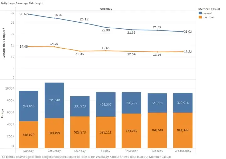

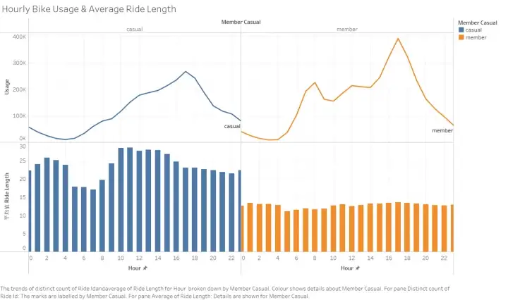
- Generally, the average ride length of casual users is usually greater than members.
- The average ride length of casual riders during weekends also increases with the usage. Bike usage steady increase in the second quarter and reached the peak at the middle of the third quarter of the year. The reason causes such trend may connect to the weather condition, the decreasing trend usually happens during winter season.
- The demand for bikes at off-office hour usually extremely high (4pm-6pm), both customers types may face insufficient access to bikes.
Share
To convert casual users into annual members, the market team can adopt serval corresponding strategies with recommendations below.
- Start the marketing campaign in earlier June to prepare for the peak season, and the advertisements dropping would be targeted to the most popular stations.
- It is better to offer seasonal discounts for summer seasons or weekend riding discounts for members, and further provide a larger discount for users who decided to maintain their status membership.
- Adding a function such as a booking system exclusively for members, to help them secure a bike during busy hours.

Thank you for taking time to read my project, please leave comments for anything I can improve, Hooyah!
